So far, we have primarily considered quantitative variables in our regression models: wages measured in dollars, years of education, birthweight in grams, and so on. But in empirical work, some of the most important variables are qualitative: race, gender, region, industry, or whether someone participated in a program. This chapter introduces techniques for incorporating categorical information into regression models and for modeling non-linear relationships.
7.1 Categorical Variables in Regression
Regression requires numeric inputs, so we cannot simply include a variable like “region” with values “South,” “Midwest,” “Northeast,” and “West” directly in our model. We need a way to translate qualitative information into numbers.
7.1.1 Dummy Variables
The most common approach is to create dummy variables (also called binary or indicator variables). A dummy variable takes only two values: 1 if the observation has a particular characteristic, and 0 otherwise.
Consider this simple example from the Star Wars dataset:
The species variable is qualitative—we cannot use it directly in a regression. But we can create a dummy variable called human that equals 1 for humans and 0 for droids:
Now we have a numeric variable that captures whether each character is human.
7.1.2 Interpreting Dummy Variable Coefficients
To see how dummy variables work in regression, let’s examine a practical example. Suppose we want to know whether taking calculus in high school affects performance in college economics courses. We have data on students’ economics exam scores, their high school GPA, and whether they took calculus.
where calculus equals 1 if the student took calculus and 0 otherwise.
lm1 <-lm(score ~ hsgpa + calculus, data = wooldridge::econmath)summary(lm1)
Call:
lm(formula = score ~ hsgpa + calculus, data = wooldridge::econmath)

Residuals:
    Min      1Q  Median      3Q     Max
-54.355  -7.457   1.148   8.699  29.825

Coefficients:
            Estimate Std. Error t value             Pr(>|t|)
(Intercept)  24.5276     4.0759   6.018       0.000000002624 ***
hsgpa        13.2038     1.2257  10.772 < 0.0000000000000002 ***
calculus      5.8243     0.8992   6.477       0.000000000158 ***
---
Signif. codes:  0 '***' 0.001 '**' 0.01 '*' 0.05 '.' 0.1 ' ' 1

Residual standard error: 12.18 on 853 degrees of freedom
Multiple R-squared:  0.1756,    Adjusted R-squared:  0.1737
F-statistic: 90.87 on 2 and 853 DF,  p-value: < 0.00000000000000022
How do we interpret these coefficients? The coefficient on hsgpa (\(\hat{\beta}_1 \approx 13.2\)) tells us that a one-point increase in high school GPA is associated with about a 13-point increase in economics score, holding calculus status constant.
The coefficient on calculus (\(\hat{\beta}_2 \approx 5.8\)) tells us that students who took calculus score about 5.8 points higher on average than students who did not, holding GPA constant. This is the difference in intercepts between the two groups.
7.1.3 Visualizing What Dummy Variables Do
To understand what’s happening geometrically, think about the regression line for each group.
For students who did not take calculus (calculus = 0): \[
\widehat{score} = \hat{\beta}_0 + \hat{\beta}_1(hsgpa) + \hat{\beta}_2(0) = \hat{\beta}_0 + \hat{\beta}_1(hsgpa)
\]
For students who did take calculus (calculus = 1): \[
\widehat{score} = \hat{\beta}_0 + \hat{\beta}_1(hsgpa) + \hat{\beta}_2(1) = (\hat{\beta}_0 + \hat{\beta}_2) + \hat{\beta}_1(hsgpa)
\]
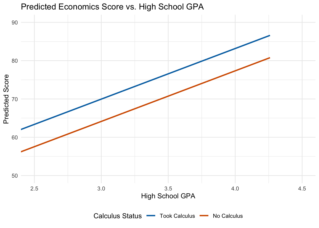
Both groups have the same slope (\(\hat{\beta}_1\)), but the calculus group has a higher intercept by exactly \(\hat{\beta}_2\). The dummy variable shifts the regression line up or down:
Figure 7.1: Dummy variables shift the intercept while keeping the slope constant.
ImportantKey Insight
A dummy variable coefficient represents the difference in intercepts between groups. Both groups share the same slope—the effect of increasing \(x\) by one unit is the same regardless of group membership.
7.2 The Dummy Variable Trap
You might wonder: why not include dummy variables for both calculus-takers and non-calculus-takers? In other words, why not estimate:
The problem is that this creates perfect multicollinearity. For every student in the dataset: \[
calculus + no\_calculus = 1
\]
This means \(no\_calculus = 1 - calculus\), so one variable is a perfect linear function of the other. OLS cannot separately identify the effects of perfectly collinear variables.
This is called the dummy variable trap. To avoid it, we always omit one category. The omitted category becomes our baseline or reference group, and all coefficients are interpreted relative to this baseline.
In our example, non-calculus-takers are the baseline. The coefficient \(\hat{\beta}_2 = 5.8\) means calculus-takers score 5.8 points higher than non-calculus-takers.
7.3 Multiple Categories
What if our categorical variable has more than two values? Consider the Palmer Penguins data, where species can be Adelie, Chinstrap, or Gentoo.
To include species in a regression, we create \(g - 1\) dummy variables where \(g\) is the number of categories. With three species, we need two dummy variables:
Call:
lm(formula = flipper_length_mm ~ body_mass_g + species_Chinstrap +
    species_Gentoo, data = penguin_data)

Residuals:
     Min       1Q   Median       3Q      Max
-14.5455  -3.1845   0.1307   3.3533  17.5313

Coefficients:
                     Estimate  Std. Error t value             Pr(>|t|)
(Intercept)       158.8602606   2.3865767  66.564 < 0.0000000000000002 ***
body_mass_g         0.0084021   0.0006339  13.255 < 0.0000000000000002 ***
species_Chinstrap   5.5974403   0.7882166   7.101     0.00000000000733 ***
species_Gentoo     15.6774699   1.0906591  14.374 < 0.0000000000000002 ***
---
Signif. codes:  0 '***' 0.001 '**' 0.01 '*' 0.05 '.' 0.1 ' ' 1

Residual standard error: 5.395 on 338 degrees of freedom
  (2 observations deleted due to missingness)
Multiple R-squared:  0.8541,    Adjusted R-squared:  0.8528
F-statistic: 659.4 on 3 and 338 DF,  p-value: < 0.00000000000000022
Interpretation:
\(\hat{\beta}_1 \approx 0.008\): A 1-gram increase in body mass is associated with a 0.008 mm increase in flipper length, holding species constant.
\(\hat{\beta}_2 \approx 5.6\): Chinstrap penguins have flippers about 5.6 mm longer than Adelie penguins of the same body mass.
\(\hat{\beta}_3 \approx 15.7\): Gentoo penguins have flippers about 15.7 mm longer than Adelie penguins of the same body mass.
7.3.1 Choosing the Baseline Category
How should we choose which category to omit? It depends on our research question.
If we only care about controlling for the categorical variable (not interpreting its coefficients), then the choice doesn’t matter—the coefficient on our main variable of interest won’t change.
If we do care about interpreting the dummy coefficients, choose a baseline that makes interpretation natural. For studying the gender wage gap, making “male” the baseline means the female coefficient directly measures the wage gap relative to men.
Let’s verify that changing the baseline doesn’t affect other coefficients:
# Switching baseline to Gentoopenguin_data <- penguin_data |>mutate(species_Adelie =case_when(species =="Adelie"~1, TRUE~0))lm_penguin2 <-lm(flipper_length_mm ~ body_mass_g + species_Chinstrap + species_Adelie, data = penguin_data)# Compare body mass coefficientscat("Body mass coefficient (Adelie baseline):", round(coef(lm_penguin)["body_mass_g"], 5), "\n")
Body mass coefficient (Adelie baseline): 0.0084
cat("Body mass coefficient (Gentoo baseline):", round(coef(lm_penguin2)["body_mass_g"], 5))
Body mass coefficient (Gentoo baseline): 0.0084
The coefficient on body mass is identical regardless of which species is the baseline.
7.4 Factor Variables in R
Creating dummy variables manually is tedious, especially when categories are numerous. R’s factor variables automate this process.
When you include a factor variable in a regression, R automatically creates the necessary dummy variables and omits one category:
# Convert species to factorpenguin_data <- penguins |>mutate(species_f =factor(species))# R handles dummy creation automaticallylm_factor <-lm(flipper_length_mm ~ body_mass_g + species_f, data = penguin_data)summary(lm_factor)
Call:
lm(formula = flipper_length_mm ~ body_mass_g + species_f, data = penguin_data)

Residuals:
     Min       1Q   Median       3Q      Max
-14.5455  -3.1845   0.1307   3.3533  17.5313

Coefficients:
                      Estimate  Std. Error t value             Pr(>|t|)
(Intercept)        158.8602606   2.3865767  66.564 < 0.0000000000000002 ***
body_mass_g          0.0084021   0.0006339  13.255 < 0.0000000000000002 ***
species_fChinstrap   5.5974403   0.7882166   7.101     0.00000000000733 ***
species_fGentoo     15.6774699   1.0906591  14.374 < 0.0000000000000002 ***
---
Signif. codes:  0 '***' 0.001 '**' 0.01 '*' 0.05 '.' 0.1 ' ' 1

Residual standard error: 5.395 on 338 degrees of freedom
  (2 observations deleted due to missingness)
Multiple R-squared:  0.8541,    Adjusted R-squared:  0.8528
F-statistic: 659.4 on 3 and 338 DF,  p-value: < 0.00000000000000022
Notice the coefficients are identical to our manual approach. R chose “Adelie” as the baseline because it comes first alphabetically.
To change the baseline category, use the relevel() function:
# Make Gentoo the baselinepenguin_data <- penguin_data |>mutate(species_f =relevel(species_f, ref ="Gentoo"))lm_factor2 <-lm(flipper_length_mm ~ body_mass_g + species_f, data = penguin_data)summary(lm_factor2)
Call:
lm(formula = flipper_length_mm ~ body_mass_g + species_f, data = penguin_data)

Residuals:
     Min       1Q   Median       3Q      Max
-14.5455  -3.1845   0.1307   3.3533  17.5313

Coefficients:
                      Estimate  Std. Error t value             Pr(>|t|)
(Intercept)        174.5377305   3.2542422  53.634 < 0.0000000000000002 ***
body_mass_g          0.0084021   0.0006339  13.255 < 0.0000000000000002 ***
species_fAdelie    -15.6774699   1.0906591 -14.374 < 0.0000000000000002 ***
species_fChinstrap -10.0800297   1.1787380  -8.552 0.000000000000000428 ***
---
Signif. codes:  0 '***' 0.001 '**' 0.01 '*' 0.05 '.' 0.1 ' ' 1

Residual standard error: 5.395 on 338 degrees of freedom
  (2 observations deleted due to missingness)
Multiple R-squared:  0.8541,    Adjusted R-squared:  0.8528
F-statistic: 659.4 on 3 and 338 DF,  p-value: < 0.00000000000000022
Now coefficients are relative to Gentoo penguins.
7.5 Non-Linear Relationships: Polynomial Models
So far we’ve assumed linear relationships between variables. But many economic relationships are non-linear. Consider the effect of work experience on wages: at low experience levels, additional experience substantially increases productivity and wages; but at very high experience levels, workers may become less productive as they age.
This suggests a quadratic relationship—wages increase with experience at first, then eventually decrease. A quadratic model takes the general form:
\[
Y = \beta_0 + \beta_1 X + \beta_2 X^2 + \mu
\]
This is called a “quadratic” because it includes \(X\) raised to the second power (\(X^2\)). Recall from algebra that the graph of a quadratic function is a parabola—a U-shape or an inverted-U shape. The sign of \(\beta_2\) determines the shape: if \(\beta_2 > 0\), the parabola opens upward (U-shaped); if \(\beta_2 < 0\), the parabola opens downward (inverted-U or “hump” shaped).
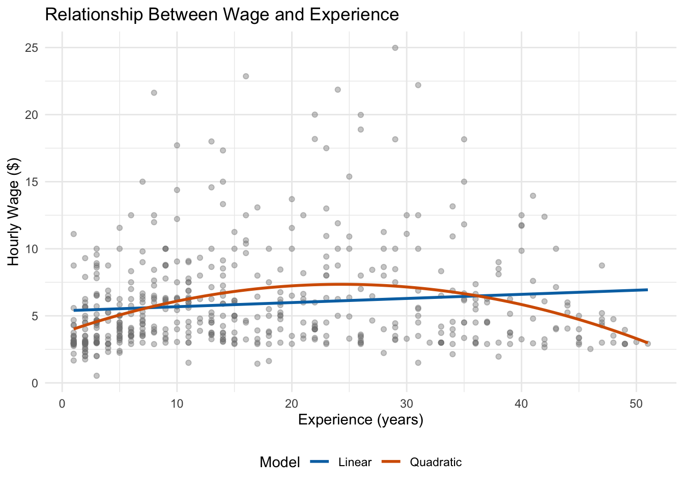
For the experience-wage relationship, we would expect \(\beta_2 < 0\): wages rise with experience early in a career but eventually level off or decline. Let’s see how a quadratic compares to a simple linear model:
Figure 7.2: A quadratic model (orange) captures the curvature in the experience-wage relationship that a linear model (blue) misses.
Notice in Figure 7.2 that the linear model predicts a constant increase in wages for every additional year of experience. The quadratic model, by contrast, curves—it captures the fact that wages rise steeply at first and then flatten out. This is a much more realistic representation of the data.
7.5.1 Estimating Quadratic Models
To estimate a quadratic model, we simply include both the variable and its square as regressors. For our wage-experience example, the model is:
Call:
lm(formula = wage ~ exper + exper2, data = wage_data)

Residuals:
    Min      1Q  Median      3Q     Max
-5.5916 -2.1440 -0.8603  1.1801 17.7649

Coefficients:
              Estimate Std. Error t value             Pr(>|t|)
(Intercept)  3.7254058  0.3459392  10.769 < 0.0000000000000002 ***
exper        0.2981001  0.0409655   7.277     0.00000000000126 ***
exper2      -0.0061299  0.0009025  -6.792     0.00000000003015 ***
---
Signif. codes:  0 '***' 0.001 '**' 0.01 '*' 0.05 '.' 0.1 ' ' 1

Residual standard error: 3.524 on 523 degrees of freedom
Multiple R-squared:  0.09277,   Adjusted R-squared:  0.0893
F-statistic: 26.74 on 2 and 523 DF,  p-value: 0.000000000008774
Notice that both exper and exper2 appear in the model. The positive coefficient on exper and the negative coefficient on exper2 confirm the inverted-U shape we saw in the figure: wages increase with experience at first, but at a decreasing rate.
7.5.2 Interpreting Quadratic Models
With a quadratic term, the marginal effect of \(X\) on \(Y\) is no longer constant—it changes depending on the current value of \(X\). This is the key difference from a linear model, where the marginal effect is always \(\beta_1\) regardless of where you are.
To find the marginal effect in a quadratic model, we take the derivative of \(Y\) with respect to \(X\):
\[
\frac{\partial Y}{\partial X} = \beta_1 + 2\beta_2 X
\]
The effect of one more year of experience depends on how much experience you already have.
Using our estimates (\(\hat{\beta}_1 \approx 0.298\), \(\hat{\beta}_2 \approx -0.006\)):
For a worker with 5 years of experience: \[
0.298 + 2(-0.006)(5) = 0.298 - 0.06 = 0.238
\] An additional year of experience is associated with a $0.24 increase in hourly wages.
For a worker with 25 years of experience: \[
0.298 + 2(-0.006)(25) = 0.298 - 0.30 = -0.002
\] An additional year of experience has essentially zero effect on wages—this worker is near the peak.
For a worker with 40 years of experience: \[
0.298 + 2(-0.006)(40) = 0.298 - 0.48 = -0.182
\] An additional year actually decreases wages by about $0.18—the worker is past the peak of the experience-wage relationship.
NoteFinding the Peak
The experience level where wages are maximized occurs where the marginal effect equals zero: \[
\beta_1 + 2\beta_2 x^* = 0 \implies x^* = -\frac{\beta_1}{2\beta_2}
\]
With our estimates: \(x^* = -\frac{0.298}{2(-0.006)} \approx 24.8\) years. This tells us that, according to our model, wages peak at about 25 years of experience.
Up to this point, all of our regression models have used variables in their original units—dollars, years, grams, and so on. But economists very frequently use the natural logarithm (denoted \(\ln\) or \(\log\)) to transform variables before putting them into a regression. Why would we do this?
There are two main motivations. First, many economic variables—like wages, income, prices, and population—are right-skewed: most observations cluster at lower values, but a long tail stretches to the right. Taking the log “compresses” this tail and makes the distribution more symmetric, which often produces a better-fitting model. Second, and more importantly for interpretation, using logs lets us talk about percentage changes rather than absolute changes, which is often more economically meaningful. A $1 raise means very different things to someone earning $10/hour versus $100/hour, but a 10% raise is comparable across both.
7.6.1 Quick Review: What Is a Logarithm?
Recall that the natural logarithm is the inverse of the exponential function. If \(e^a = b\), then \(\ln(b) = a\), where \(e \approx 2.718\).
A key property that makes logs so useful in regression is:
This means that the difference in logs is closely related to the percentage change. Specifically, for small changes:
\[
\ln(Y_1) - \ln(Y_0) \approx \frac{Y_1 - Y_0}{Y_0} = \text{proportional change in } Y
\]
This approximation works because of a calculus result: the derivative of \(\ln(Y)\) with respect to \(Y\) is \(1/Y\), so \(d\ln(Y) = dY/Y\)—a small change in the log of \(Y\) equals the proportional change in \(Y\) itself. Multiplying by 100 gives us the percent change.
NoteWhy This Approximation Works
Consider a wage increase from $20 to $21. The proportional change is \((21-20)/20 = 0.05\), or 5%. The difference in logs is \(\ln(21) - \ln(20) = 3.045 - 2.996 = 0.049\), which is very close to 0.05.
But for larger changes the approximation gets worse. A change from $20 to $30 is a 50% increase, but \(\ln(30) - \ln(20) = 0.405\), not 0.50. We’ll discuss what to do about larger changes below.
7.6.2 Log-Linear Models
The most common log transformation in applied economics is to log only the dependent variable. This gives us the log-linear model:
\[
\ln(Y) = \beta_0 + \beta_1 X + \mu
\]
Here the left-hand side is in logs but the right-hand side variable \(X\) is in its original units (levels).
Deriving the interpretation. To see why logs change the interpretation, suppose \(X\) increases by one unit (from \(X_0\) to \(X_0 + 1\)), holding everything else constant. Then:
Now recall that \(\ln(Y_1) - \ln(Y_0) \approx (Y_1 - Y_0)/Y_0\) for small changes. So:
\[
\frac{Y_1 - Y_0}{Y_0} \approx \beta_1
\]
Multiplying both sides by 100:
\[
\text{Percent change in } Y \approx 100 \times \beta_1
\]
Interpretation: A one-unit increase in \(X\) is associated with an approximately \(100 \times \beta_1\) percent change in \(Y\).
Let’s see this in action with our wage data. We’ll estimate a model with log wages as the dependent variable and education as the independent variable:
lm_loglin <-lm(log(wage) ~ educ, data = wooldridge::wage1)summary(lm_loglin)
Call:
lm(formula = log(wage) ~ educ, data = wooldridge::wage1)

Residuals:
     Min       1Q   Median       3Q      Max
-2.21158 -0.36393 -0.07263  0.29712  1.52339

Coefficients:
            Estimate Std. Error t value             Pr(>|t|)
(Intercept) 0.583773   0.097336   5.998        0.00000000374 ***
educ        0.082744   0.007567  10.935 < 0.0000000000000002 ***
---
Signif. codes:  0 '***' 0.001 '**' 0.01 '*' 0.05 '.' 0.1 ' ' 1

Residual standard error: 0.4801 on 524 degrees of freedom
Multiple R-squared:  0.1858,    Adjusted R-squared:  0.1843
F-statistic: 119.6 on 1 and 524 DF,  p-value: < 0.00000000000000022
The coefficient on educ is approximately 0.083. Multiplying by 100 gives 8.3. So we interpret this as: an additional year of education is associated with approximately an 8.3% increase in hourly wages.
Notice how different this is from a level-level model, where we would say “an additional year of education is associated with a $X increase in wages.” The percentage interpretation is arguably more natural for wages, since a $1 raise means different things at different wage levels.
WarningWhen the Approximation Breaks Down
The “\(100 \times \beta_1\) percent” interpretation is an approximation that works well when \(\beta_1\) is small—roughly when \(|\beta_1| < 0.20\).
For larger coefficients, the approximation becomes inaccurate. In those cases, use the exact formula:
For example, if \(\hat{\beta}_1 = 0.40\), the approximate interpretation would be a 40% change, but the exact calculation gives \(100 \times (e^{0.40} - 1) = 100 \times (1.492 - 1) = 49.2\%\). That’s a meaningful difference!
This exact formula is particularly important when interpreting dummy variable coefficients in log-linear models, since those coefficients are often large enough for the approximation to be poor.
7.6.3 Linear-Log Models
We can also log an independent variable while keeping the dependent variable in levels:
\[
Y = \beta_0 + \beta_1 \ln(X) + \mu
\]
Deriving the interpretation. Now suppose \(X\) increases by 1% (i.e., \(X\) goes from \(X_0\) to \(1.01 \times X_0\)). The change in \(\ln(X)\) is:
So a 1% change in \(X\) changes \(\ln(X)\) by approximately 0.01. The resulting change in \(Y\) is:
\[
\Delta Y = \beta_1 \times 0.01 = \frac{\beta_1}{100}
\]
Interpretation: A 1% increase in \(X\) is associated with a \(\beta_1 / 100\) unit change in \(Y\).
This functional form is useful when \(X\) varies over a wide range and we believe that proportional changes in \(X\) matter more than absolute changes. For instance, if we regress birthweight in grams on the log of family income, a 1% increase in income might be associated with a \(\beta_1/100\)-gram increase in birthweight—regardless of whether the family earns $20,000 or $200,000.
bwght_data <- wooldridge::bwght |>filter(faminc >0) # drop zeros since log(0) is undefinedlm_linlog <-lm(bwght ~log(faminc), data = bwght_data)summary(lm_linlog)
Call:
lm(formula = bwght ~ log(faminc), data = bwght_data)

Residuals:
    Min      1Q  Median      3Q     Max
-95.799 -11.799   0.621  13.014 150.708

Coefficients:
            Estimate Std. Error t value             Pr(>|t|)
(Intercept) 111.4881     1.8982  58.735 < 0.0000000000000002 ***
log(faminc)   2.3481     0.5922   3.965            0.0000771 ***
---
Signif. codes:  0 '***' 0.001 '**' 0.01 '*' 0.05 '.' 0.1 ' ' 1

Residual standard error: 20.25 on 1386 degrees of freedom
Multiple R-squared:  0.01122,   Adjusted R-squared:  0.0105
F-statistic: 15.72 on 1 and 1386 DF,  p-value: 0.00007708
The coefficient on log(faminc) is approximately 2.47. This means a 1% increase in family income is associated with a \(2.47/100 = 0.025\) ounce increase in birthweight. Or equivalently, a 10% increase in family income is associated with about a 0.25 ounce increase in birthweight.
7.6.4 Log-Log Models (Elasticities)
When both sides are logged:
\[
\ln(Y) = \beta_0 + \beta_1 \ln(X) + \mu
\]
Deriving the interpretation. A 1% increase in \(X\) changes \(\ln(X)\) by approximately 0.01 (as we derived above). The change in \(\ln(Y)\) is then:
\[
\Delta \ln(Y) = \beta_1 \times 0.01
\]
Since \(\Delta \ln(Y) \approx\) proportional change in \(Y\), multiplying by 100:
\[
\text{Percent change in } Y \approx \beta_1 \times 0.01 \times 100 = \beta_1 \times 1\%
\]
So: a 1% increase in \(X\) is associated with a \(\beta_1\)% change in \(Y\).
Interpretation:\(\beta_1\) is the elasticity of \(Y\) with respect to \(X\)—a unit-free measure of how responsive \(Y\) is to changes in \(X\). Elasticities are a cornerstone of economics. If \(\beta_1 = -0.5\), for example, we would say that \(Y\) is “inelastic” with respect to \(X\)—a 1% increase in \(X\) leads to only a 0.5% decrease in \(Y\).
wage_educ <- wooldridge::wage1 |>filter(educ >0) # drop zeros since log(0) is undefinedlm_loglog <-lm(log(wage) ~log(educ), data = wage_educ)summary(lm_loglog)
Call:
lm(formula = log(wage) ~ log(educ), data = wage_educ)

Residuals:
     Min       1Q   Median       3Q      Max
-2.24076 -0.38426 -0.05421  0.32273  1.49421

Coefficients:
            Estimate Std. Error t value            Pr(>|t|)
(Intercept) -0.44468    0.21785  -2.041              0.0417 *
log(educ)    0.82521    0.08645   9.546 <0.0000000000000002 ***
---
Signif. codes:  0 '***' 0.001 '**' 0.01 '*' 0.05 '.' 0.1 ' ' 1

Residual standard error: 0.4913 on 522 degrees of freedom
Multiple R-squared:  0.1486,    Adjusted R-squared:  0.147
F-statistic: 91.12 on 1 and 522 DF,  p-value: < 0.00000000000000022
The coefficient is approximately 0.825, meaning a 1% increase in education is associated with approximately a 0.825% increase in wages. Education and wages are inelastic in this specification—a 1% increase in education corresponds to less than a 1% increase in wages.
7.6.5 When to Use Logs
There are no hard-and-fast rules, but here are some practical guidelines:
Variables that are commonly logged include wages, income, prices, population, firm size (revenue, employees), and expenditures. These tend to be strictly positive, right-skewed, and best thought of in percentage terms.
Variables that are typically not logged include years of education, age, percentages or rates (unemployment rate, graduation rate), dummy variables, and variables that can take zero or negative values (since the log of zero or a negative number is undefined).
TipPractical Advice
When in doubt, try plotting the variable. If its distribution is right-skewed and the variable is strictly positive, logging it is often a good idea. You can also compare the \(R^2\) of models with and without the log transformation—though model fit alone shouldn’t be the sole criterion. The most important consideration is whether the interpretation makes economic sense.
7.7 Application: Policy Evaluation with Dummy Variables
Dummy variables are essential for evaluating policies and programs. Suppose we want to estimate the effect of a job training program on wages:
where training equals 1 if the person participated in the program and 0 otherwise.
The coefficient \(\beta_1\) measures the treatment effect—the percentage difference in wages between program participants and non-participants, controlling for education and experience. Since the dependent variable is logged, we multiply \(\beta_1\) by 100 to get the approximate percentage effect (or use the exact formula \(100 \times (e^{\beta_1} - 1)\) for larger coefficients).
This is essentially a regression-based version of comparing treatment and control groups, where the control variables help us account for differences between those who did and didn’t participate.
7.8 Functional Form Interpretation Reference
The table below summarizes how to interpret \(\beta_1\) under each functional form we have covered. This is one of the most important references in the course—you should be able to quickly identify the correct interpretation for any model you encounter.
Table 7.1: Functional Form Interpretation Guide
Model
Equation
Interpretation of \(\hat{\beta}_1\)
Example
Level-Level
\(Y = \beta_0 + \beta_1 X\)
A 1-unit increase in \(X\) → \(\beta_1\)-unit change in \(Y\)
\(wage = 2.1 + 0.54 \cdot educ\): one more year of education → $0.54 higher wages
Log-Level
\(\ln(Y) = \beta_0 + \beta_1 X\)
A 1-unit increase in \(X\) → \((100 \times \beta_1)\)% change in \(Y\)
\(\ln(wage) = 0.58 + 0.083 \cdot educ\): one more year of education → ≈ 8.3% higher wages
Level-Log
\(Y = \beta_0 + \beta_1 \ln(X)\)
A 1% increase in \(X\) → \(\beta_1 / 100\) unit change in \(Y\)
\(bwght = 116.1 + 2.47 \cdot \ln(faminc)\): 1% higher income → 0.025 oz higher birthweight
Log-Log
\(\ln(Y) = \beta_0 + \beta_1 \ln(X)\)
A 1% increase in \(X\) → \(\beta_1\)% change in \(Y\) (elasticity)
\(D=1\) group has ≈ \((100 \times \beta_1)\)% different \(Y\). Exact: \(100(e^{\beta_1}-1)\)%
\(\ln(wage) = 1.0 - 0.15 \cdot female\): women earn ≈ 15% less (exact: −13.9%)
TipHow to Use This Table
When you encounter a regression in a paper or problem set, the first thing to check is: is the dependent variable logged? Is the independent variable logged? Your answers determine which row of the table applies. Then use the interpretation column to state the result in plain English.
7.9 Summary
This chapter introduced two powerful extensions to basic regression: categorical variables and non-linear functional forms.
Dummy variables allow us to include qualitative information in regression models. The coefficient on a dummy variable represents the difference in intercepts between groups—the effect of having a particular characteristic relative to the baseline category. When a categorical variable has \(g\) categories, we include \(g - 1\) dummy variables to avoid perfect multicollinearity (the dummy variable trap).
Polynomial models capture non-linear relationships by including squared or higher-order terms. With quadratic models, the marginal effect of \(x\) on \(y\) depends on the current level of \(x\), allowing us to model relationships that increase and then decrease (or vice versa).
Logarithmic transformations change the interpretation of coefficients. The key insight is that a change in a logged variable approximates a proportional (percentage) change. Log-linear models give the percentage change in \(Y\) for a one-unit change in \(X\); linear-log models give the unit change in \(Y\) for a one-percent change in \(X\); and log-log models give elasticities—the percentage change in \(Y\) for a one-percent change in \(X\). These transformations are especially useful when dealing with variables like wages or prices that are right-skewed and where percentage changes are more meaningful than absolute changes. See Table 7.1 for a complete reference.
7.10 Check Your Understanding
For each question below, select the best answer from the dropdown menu. The dropdown will turn green if correct and red if incorrect.
TipShow Explanation
With a log-linear model (log on the left side only), we multiply the coefficient by 100 to get the percentage interpretation. A coefficient of -0.15 means women earn approximately 15% less than men (the baseline category), holding other variables constant.
If we include dummy variables for all g categories plus an intercept, the dummy variables will sum to 1 for every observation, creating perfect collinearity with the intercept. This is the “dummy variable trap.” Omitting one category solves this problem.
A negative coefficient on the squared term means the parabola opens downward. Combined with a positive coefficient on the linear term, this creates an inverted-U shape: wages increase with experience initially, but at a decreasing rate, and eventually begin to decline.
In a log-log model, both variables are in logs, so the coefficient is an elasticity. It tells us the percentage change in Y for a 1% change in X. Here, a 1% increase in X is associated with a 0.5% increase in Y.
Changing the baseline category changes how the dummy coefficients are interpreted (they become relative to a different group), but it doesn’t affect coefficients on other variables in the model. The model’s predictions and fit remain identical.
The experience level that maximizes wages is found by setting the derivative equal to zero: 0.30 + 2(-0.006)(exper) = 0. Solving: exper = 0.30/(2 × 0.006) = 0.30/0.012 = 25 years.
Bailey, Michael A. 2020. Real Econometrics: The Right Tools to Answer Important Questions. Oxford University Press.
Wooldridge, Jeffrey M. 2019. Introductory Econometrics: A Modern Approach. 7th ed. Cengage Learning.