14  Instrumental Variables

TipKey Questions

• What is endogeneity and why does it cause OLS to fail?
• What are instrumental variables and what makes an instrument valid?
• How does Two-Stage Least Squares (2SLS) work?
• What is the Local Average Treatment Effect (LATE)?
• How do we test whether an instrument is strong enough?

NoteSuggested Readings

• TBD

We’ve built up a powerful toolkit for causal inference: randomized experiments, multivariate regression, fixed effects, and difference-in-differences. But what happens when none of these methods are available?

Sometimes we have only cross-sectional data, treatment is clearly endogenous, we cannot randomize, and there’s no natural experiment to exploit. In these situations, instrumental variables (IV) offers a path forward—if we can find the right instrument.

14.1 The Fundamental Problem: Endogeneity

14.1.1 When OLS Fails

Recall that OLS provides unbiased estimates when the zero conditional mean assumption holds: \(E[\mu | X] = 0\). When this assumption fails—when \(X\) is correlated with the error term—we say \(X\) is endogenous, and OLS is biased.

Endogeneity arises from three main sources:

1. Omitted Variable Bias

We spent a lot of time discussing this in Chapter 5. We want to estimate the effect of education on wages, but ability affects both education choices and wages. Since we can’t measure ability, it’s absorbed into the error term, biasing our estimate.

2. Selection Bias

We want to estimate the effect of health insurance on health outcomes, but healthier people are more likely to purchase insurance. Health status drives insurance decisions, contaminating our comparison.

3. Reverse Causality

We want to estimate the effect of police on crime, but high-crime areas get more police deployed. The causation runs both ways, making it impossible to isolate the effect of policing.

If we have any of these problems in our regression, we cannot interpret the OLS coefficient as a causal effect.

14.2 The Instrumental Variables Solution

14.2.1 Endogenous vs. Exogenous Variation

If we are worried that our OLS estimate is biased, and that our independent variable \(X\) is endogenous, then we have a problem.

The IV solution is to try to find an exogenous source of variation in \(X\), which we can then use to learn about the causal effect of \(X\) on \(y\).

In other words, the IV approach finds a variable \(Z\), the instrument, that “shakes up” \(X\) in a way that’s unrelated to the error term. Think of it as finding a source of exogenous variation in \(X\)—variation that comes from outside the system and isn’t contaminated by the factors causing endogeneity.

14.2.2 Two Requirements for a Valid Instrument

So how do we find a variable \(Z\) that would work as our instrument?

For \(Z\) to be a valid instrument, it must satisfy two conditions:

ImportantThe Two IV Assumptions

1. Relevance: \(Cov(Z, X) \neq 0\)

The instrument must be correlated with the endogenous variable. This is testable—we can check whether \(Z\) predicts \(X\).

2. Exclusion Restriction: \(Cov(Z, \mu) = 0\)

The instrument affects \(Y\) only through \(X\). There is no direct effect of \(Z\) on \(Y\). This is not directly testable—it requires economic reasoning and assumption.

If either of these requirements fails, then our instrument \(Z\) does not successfully isolate the exogenous variation in \(X\), and our IV estimate will still be partially contaminated by the same bias OLS suffers from.

14.2.3 A Running Example: Fertility and Maternal Labor Supply

Abstract letters are a lot easier to swallow when they are pinned to a real study, so before we draw the diagram, let’s introduce the empirical application we will keep coming back to.

The research question. What is the causal effect of having an additional child on a mother’s labor force participation? This is a first-order question for understanding the gender wage gap, designing parental leave policy, and evaluating childcare subsidies. But we obviously cannot randomize fertility, and the decision to have children is deeply endogenous:

• Reverse causality: women may time fertility around their careers.
• Selection: women who are less career-oriented may choose larger families.
• Omitted variables: unobserved preferences drive both fertility and work.

Regressing a mother’s employment on her number of children by OLS tangles all of these forces together with the causal effect we actually want.

Angrist and Evans (1998) found a clever instrument for fertility: the sex composition of the first two children. The idea is that parents tend to prefer a mix of sexes among their children. Families whose first two children are the same sex (i.e., two boys or two girls) are more likely to try for a third child to “get” the other sex than families whose first two children are already one of each. Since the assigned sex at birth of a child is essentially biological chance, having same-sex versus mixed-sex first two children is essentially random.

Translating this study into the language of the two IV assumptions:

• Relevance (\(\text{Cov}(Z, X) \neq 0\)): parents of same-sex siblings (\(Z\)) are measurably more likely to have a third child (\(X\)). This is an empirical fact we can (and will) verify in the data.
• Exclusion (\(\text{Cov}(Z, \mu) = 0\)): the sex mix of a woman’s first two children (\(Z\)) is plausibly uncorrelated with her unobserved career orientation, her husband’s earnings, or anything else that would shape her labor supply (\(\mu\)) except through its effect on fertility (\(X\)).

14.2.4 Graphical Intuition

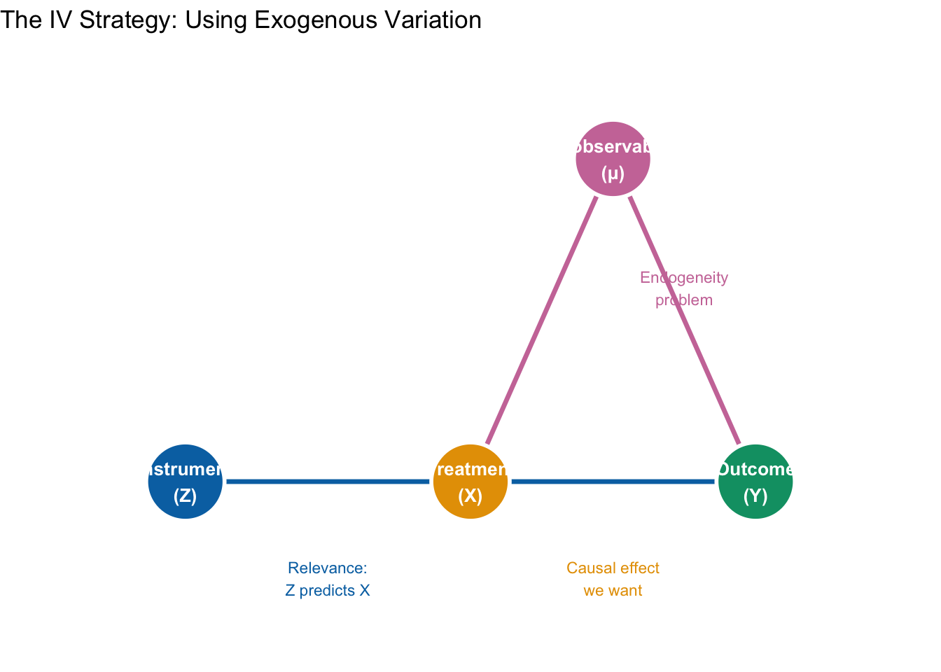
The cleanest way to see why IV works is with a causal diagram (a directed acyclic graph, or DAG). A DAG represents variables as nodes and causal relationships as arrows. Figure 14.1 maps the four ingredients of the Angrist-Evans design onto the four generic roles every IV application has: an instrument \(Z\) (here, same-sex first two children), an endogenous treatment \(X\) (here, having a third child), an outcome \(Y\) (here, the mother’s labor force participation), and a set of unobserved confounders \(\mu\) (here, career orientation and similar preferences).

Figure 14.1: The instrumental variables DAG. Solid blue arrows trace the identified pathway: Z moves X (the first stage), and X causes Y (the effect we want). Dashed red arrows show the confounding pathway from unobservables (μ) that makes X endogenous in the first place. The crossed-out gray arrow marks the exclusion restriction: Z must have no direct effect on Y. IV recovers β by isolating the movement in X that can be traced back to Z.

What makes this a valid IV design has less to do with which arrows are drawn than with which arrows are deliberately missing. Let’s walk through each of the five claims the diagram is making, starting from Angrist-Evans and pulling out the general principle each time.

1. \(Z \to X\): the first stage. Same-sex first two children (\(Z\)) push some families to have a third child (\(X\)). In general terms, this is the relevance condition, \(\text{Cov}(Z, X) \neq 0\): the instrument must actually move the treatment around. If this arrow is missing or nearly so—if same-sex siblings barely budged fertility— we would have a weak instrument problem, which we return to later in this chapter. This is the one IV assumption we can test directly: we will verify it shortly by comparing the share of families with three or more kids across same-sex and mixed-sex households.

2. \(X \to Y\): the causal effect we actually want. This is the arrow we care about: the effect of having a third child on a mother’s labor force participation. In generic notation, it is the parameter \(\beta\). Everything else in the diagram is infrastructure we need in order to identify this one arrow.

3. \(\mu \to X\) and \(\mu \to Y\): the endogeneity problem. These two arrows together are why OLS fails. Unobserved career orientation (\(\mu\)) affects both fertility and labor supply: strongly career-oriented women tend to have fewer children and are more likely to work, while women who prioritize family over career tend to have more children and work less. That creates a backdoor path from \(X\) back to \(Y\) running through the confounder: \(X \leftarrow \mu \to Y\). When we regress labor force participation on number of children by OLS, we cannot tell which part of the correlation comes from the \(X \to Y\) arrow we want and which part comes from the detour through \(\mu\). Concretely, OLS will make children look like they depress maternal employment more than they do, because the women who have more kids are also the women who would have worked less anyway.

4. No arrow from \(Z\) to \(Y\): the exclusion restriction. This is where the identification work actually happens. We are assuming the sex composition of the first two children has no direct effect on whether the mother works— its only pathway to labor supply runs through its effect on fertility. In generic notation, \(Z\) affects \(Y\) only through \(X\). That is why the figure draws the \(Z \to Y\) arrow in ghostly gray with a red “\(\times\)” across it: we are explicitly ruling that arrow out. This assumption is not directly testable; we have to defend it with economic reasoning. In Angrist-Evans it is defensible precisely because it is hard to tell a plausible story in which having two boys versus a boy and a girl directly changes a mother’s attachment to the labor force, except through the fertility decision it triggers.

5. No arrow from \(\mu\) to \(Z\): the instrument is exogenous. We also need the instrument itself to be uncorrelated with the unobservables: \(\text{Cov}(Z, \mu) = 0\). If career orientation influenced the sex composition of a woman’s first two children, then \(Z\) would inherit the same endogeneity it was supposed to solve. In Angrist-Evans, the sex of a child is (to a first approximation) biological chance, which is why this assumption is easy to defend here— and a big reason the paper became a canonical IV reference.

14.2.5 Why this lets us recover the causal effect

Put these five pieces together and you have the engine of IV. The instrument \(Z\) injects clean, exogenous variation into \(X\)— variation that originates outside the confounded system. IV then asks a single, disciplined question: of the movement in fertility that we can trace back to same-sex siblings, how much movement in maternal employment does it produce? Because the \(Z \to X \to Y\) pathway is the only channel through which \(Z\) can reach \(Y\), the answer to that question must be the causal effect of children on labor supply.

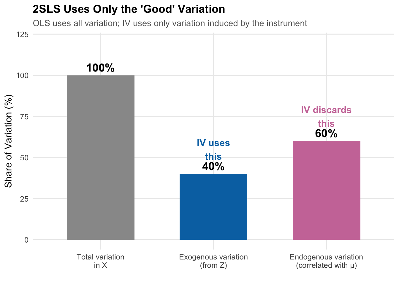
Another way to put the same idea: the treatment \(X\) has two kinds of variation. “Good” variation is the part that is unrelated to \(\mu\)— in our figure, the part induced by the \(Z \to X\) arrow. In Angrist-Evans, this is the bit of family-size variation that comes from the random sex composition of the first two children. “Bad” variation is the part correlated with \(\mu\)— in our figure, the part induced by the \(\mu \to X\) arrow. In Angrist-Evans, this is the bit of family-size variation that reflects a woman’s (unobserved) career orientation. OLS uses both kinds indiscriminately, mixing identification with contamination. IV isolates only the good variation and discards the rest, at the cost of using a smaller slice of the data to learn the answer.

14.3 Estimating IV

With the identification strategy in hand, we can now bring the Angrist-Evans design to data and actually estimate \(\beta\). We’ll work with a simulated dataset designed to mimic the Angrist-Evans structure, which has the pedagogical advantage that we know the true causal effect (we built it in) and can judge how well OLS and IV recover it.

14.3.1 Simulating the Angrist-Evans Setup

Let’s create simulated data that mirrors the Angrist-Evans setting to illustrate how IV works:

# Simulate Angrist-Evans style data
set.seed(42)
n <- 50000

# Generate data
ae_sim <- tibble(
    # Unobserved "career orientation" - affects both fertility and work
    career_orientation = rnorm(n, 0, 1),
    
    # Same-sex instrument (random)
    samesex = rbinom(n, 1, 0.5),
    
    # More than 2 kids: affected by samesex AND career orientation.
    # The 0.12 coefficient on samesex is calibrated to give a ~6 pp first-stage
    # difference (the empirical magnitude in Angrist-Evans 1998) and a first-stage
    # F well into the hundreds at n = 50,000.
    morekids_latent = -0.5 + 0.12 * samesex - 0.3 * career_orientation + rnorm(n, 0, 0.5),
    morekids = as.integer(morekids_latent > 0),
    
    # Labor force participation: affected by morekids AND career orientation
    # True causal effect of morekids is -0.10
    worked_latent = 0.6 - 0.10 * morekids + 0.25 * career_orientation + rnorm(n, 0, 0.3),
    mom_worked = as.integer(worked_latent > 0.5)
) |>
    mutate(
        samesex_lab = if_else(samesex == 1, "Same sex", "Mixed sex"),
        morekids_lab = if_else(morekids == 1, "> 2 kids", "≤ 2 kids")
    )

14.3.2 Testing the Relevance Condition

First, let’s verify that same-sex siblings predict having more than two children:

# Check relevance: does samesex predict morekids?
relevance_check <- ae_sim |>
    group_by(samesex_lab) |>
    summarize(prop_morekids = mean(morekids))

relevance_check

# A tibble: 2 × 2
  samesex_lab prop_morekids
  <chr>               <dbl>
1 Mixed sex           0.196
2 Same sex            0.258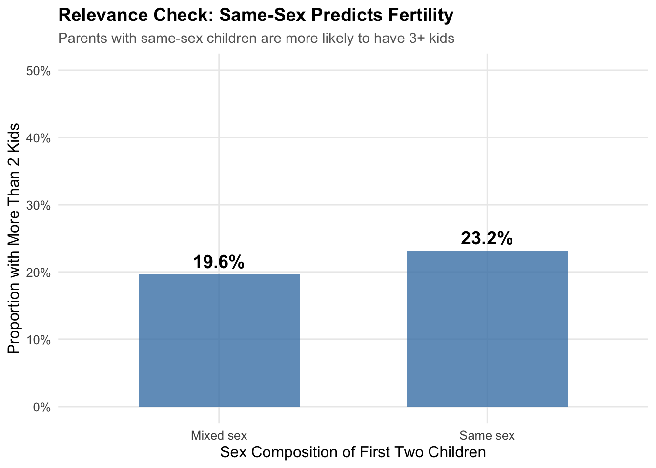

Figure 14.2: The relevance condition: parents with same-sex children are more likely to have a third child.

The difference is considerable—same-sex parents are about 6 percentage points more likely to have a third child. The instrument is relevant.

14.3.3 Testing Excludability (Sort of)

We cannot directly test the exclusion restriction, but we can check whether the instrument has a small reduced-form relationship with the outcome:

Figure 14.3: Checking excludability: the direct relationship between same-sex and labor supply is small, consistent with the effect operating through fertility.

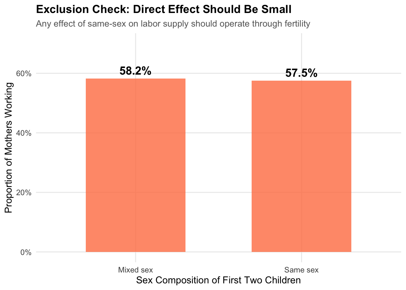
The difference is small (around a percentage point), consistent with the effect operating through fertility rather than directly. Of course, this doesn’t prove excludability—we must rely on economic reasoning to argue there’s no direct channel.

14.4 Two-Stage Least Squares (2SLS)

14.4.1 The Estimation Strategy

IV models are typically estimated using Two-Stage Least Squares (2SLS):

Stage 1 (First Stage): Regress the endogenous variable on the instrument: \[ X_i = \pi_0 + \pi_1 Z_i + \nu_i \]

Get predicted values: \(\hat{X}_i = \hat{\pi}_0 + \hat{\pi}_1 Z_i\)

These predicted values contain only the variation in \(X\) that comes from \(Z\)—the exogenous variation.

Stage 2 (Second Stage): Regress the outcome on the predicted values: \[ Y_i = \beta_0 + \beta_1 \hat{X}_i + \mu_i \]

The coefficient \(\hat{\beta}_1^{2SLS}\) is our causal estimate.

14.4.2 Why Does This Work?

The first stage “purges” \(X\) of its problematic variation. Since \(Z\) is exogenous (by assumption), the predicted values \(\hat{X}\) contain only exogenous variation. When we regress \(Y\) on \(\hat{X}\), we’re using only this “clean” variation, giving us an unbiased estimate.

Figure 14.4: 2SLS uses only the variation in X that comes from the instrument Z, discarding the endogenous variation.

14.4.3 Implementing 2SLS

Let’s estimate the model step by step:

Step 1: The First Stage

# First stage: regress endogenous variable on instrument
first_stage <- lm(morekids ~ samesex, data = ae_sim)
summary(first_stage)

Call:
lm(formula = morekids ~ samesex, data = ae_sim)

Residuals:
    Min      1Q  Median      3Q     Max 
-0.2578 -0.2578 -0.1963 -0.1963  0.8037 

Coefficients:
            Estimate Std. Error t value            Pr(>|t|)    
(Intercept) 0.196288   0.002636   74.46 <0.0000000000000002 ***
samesex     0.061536   0.003736   16.47 <0.0000000000000002 ***
---
Signif. codes:  0 '***' 0.001 '**' 0.01 '*' 0.05 '.' 0.1 ' ' 1

Residual standard error: 0.4177 on 49998 degrees of freedom
Multiple R-squared:  0.005396,  Adjusted R-squared:  0.005376 
F-statistic: 271.3 on 1 and 49998 DF,  p-value: < 0.00000000000000022

The F-statistic on samesex is very large (well into the hundreds), indicating a strong instrument.

Step 2: Get Predicted Values

# Get predicted values from first stage
ae_sim <- ae_sim |>
    mutate(morekids_hat = predict(first_stage))

# Look at the predictions
ae_sim |>
    select(samesex, morekids, morekids_hat) |>
    head(10)

# A tibble: 10 × 3
   samesex morekids morekids_hat
     <int>    <int>        <dbl>
 1       1        0        0.258
 2       0        0        0.196
 3       0        1        0.196
 4       1        0        0.258
 5       1        0        0.258
 6       1        0        0.258
 7       1        0        0.258
 8       1        0        0.258
 9       0        0        0.196
10       0        0        0.196

Step 3: The Second Stage

# Second stage: regress outcome on predicted values
# NOTE: Standard errors from this approach are WRONG
second_stage_manual <- lm(mom_worked ~ morekids_hat, data = ae_sim)
coef(second_stage_manual)["morekids_hat"]

morekids_hat 
  -0.1584669 

WarningStandard Error Warning

The manual two-stage approach gives the correct coefficient, but the standard errors are wrong because they don’t account for uncertainty in the first stage. Always use a proper 2SLS estimator that computes correct standard errors.

14.4.4 Proper 2SLS with feols()

In practice, we don’t run the two stages by hand—we use a proper 2SLS estimator that handles the standard errors correctly. The fixest package’s feols() function is the most common choice in modern applied work, and it is worth taking a few minutes to understand its syntax, because IV formulas look a bit intimidating the first time you see one.

The four-part feols() formula. For IV estimation, feols() uses a formula with three vertical bars that split the right-hand side into four pieces:

outcome ~ exogenous_controls | fixed_effects | endogenous ~ instrument(s)

Reading left to right:

• outcome: the dependent variable \(Y\) (here, mom_worked).
• exogenous_controls: any covariates you want to include that are not endogenous—age, education, region dummies, and so on. If you have no controls, put 1 for an intercept-only specification.
• fixed_effects: variables to absorb as fixed effects (e.g., state, year). Use 0 if you have none. feols() absorbs these efficiently rather than creating explicit dummies.
• endogenous ~ instrument(s): the first-stage formula. On the left is the endogenous regressor \(X\) (here, morekids); on the right are one or more instruments \(Z\) (here, samesex). feols() runs this as a separate first-stage regression internally and uses the predicted values in the second stage—but reports correct 2SLS standard errors.

Our bare-bones Angrist-Evans specification has no controls and no fixed effects, so the first two slots are filled with 1 and 0:

# Proper 2SLS estimation
# outcome    | exog. controls | fixed effects | first stage
tsls <- feols(mom_worked ~ 1  |  0             | morekids ~ samesex,
              data = ae_sim)

summary(tsls)

TSLS estimation - Dep. Var.: mom_worked
                  Endo.    : morekids
                  Instr.   : samesex
Second stage: Dep. Var.: mom_worked
Observations: 50,000
Standard-errors: IID 
              Estimate Std. Error  t value  Pr(>|t|)    
(Intercept)   0.613519   0.015972 38.41160 < 2.2e-16 ***
fit_morekids -0.158467   0.069749 -2.27196  0.023093 *  
---
Signif. codes:  0 '***' 0.001 '**' 0.01 '*' 0.05 '.' 0.1 ' ' 1
RMSE: 0.479855   Adj. R2: 7.743e-5
F-test (1st stage), morekids: stat = 271.2683, p < 2.2e-16 , on 1 and 49,998 DoF.
                  Wu-Hausman: stat =   5.9324, p = 0.014869, on 1 and 49,997 DoF.

A few things to notice in the output:

• The coefficient on fit_morekids is the 2SLS estimate of \(\beta\) (the fit_ prefix is fixest’s way of flagging that this is the fitted endogenous variable, not the raw one).
• The standard error is the correct 2SLS standard error, adjusted for the first-stage uncertainty that the manual two-step approach got wrong.
• The header reports a first-stage F-statistic (sometimes labeled “IV F-test” or “F-test (1st stage)”). This is our first diagnostic for instrument strength, which we’ll pick up in the next section.

Inspecting the first stage. feols() estimates the first stage in the background but hides it by default. To view it, pass stage = 1 to summary() (or etable() for a publication-ready table):

# Look at the first-stage regression explicitly
summary(tsls, stage = 1)

TSLS estimation - Dep. Var.: morekids
                  Endo.    : morekids
                  Instr.   : samesex
First stage: Dep. Var.: morekids
Observations: 50,000
Standard-errors: IID 
            Estimate Std. Error t value  Pr(>|t|)    
(Intercept) 0.196288   0.002636 74.4637 < 2.2e-16 ***
samesex     0.061536   0.003736 16.4702 < 2.2e-16 ***
---
Signif. codes:  0 '***' 0.001 '**' 0.01 '*' 0.05 '.' 0.1 ' ' 1
RMSE: 0.417709   Adj. R2: 0.005376
F-test (1st stage): stat = 271.27, p < 2.2e-16, on 1 and 49,998 DoF.

Adding controls. Suppose we wanted to control for the mother’s age and education. These are exogenous (we are assuming they are uncorrelated with \(\mu\)) and go in the first slot of the formula. feols() automatically includes them in both the first and second stages— exactly what 2SLS requires:

# Illustrative — not run in this chapter's data
tsls_ctrl <- feols(mom_worked ~ age + education | 0 | morekids ~ samesex,
                   data = ae_sim)

Adding fixed effects. If we wanted state fixed effects (to control for time-invariant features of states), we’d move state into the second slot:

# Illustrative
tsls_fe <- feols(mom_worked ~ age + education | state | morekids ~ samesex,
                 data = ae_sim)

feols() absorbs the fixed effects using a demeaning algorithm that is much faster than creating explicit dummies, which matters a lot on large administrative datasets.

Multiple instruments. If we had a second instrument for fertility—say, a twin-birth indicator, which Angrist and Evans also use—we’d list both on the right of the first-stage formula:

# Illustrative
tsls_multi <- feols(mom_worked ~ 1 | 0 | morekids ~ samesex + twins,
                    data = ae_sim)

The model is now overidentified (two instruments for one endogenous variable), which opens up diagnostic tests like the Sargan/Hansen overidentification test (available via fitstat(tsls_multi, ~ sargan)).

Cluster-robust standard errors. IV standard errors are sensitive to within-cluster correlation. You can cluster SEs at estimation time by passing cluster = ~ cluster_var, or after the fact with summary():

# Illustrative
summary(tsls, cluster = ~ state)

Weak-instrument diagnostics. The most important post-estimation check for IV is the first-stage F-statistic. feols() reports it in summary(), but you can pull it out directly (along with other diagnostics) with fitstat():

# Pull out IV diagnostics explicitly
fitstat(tsls, ~ ivf + ivwald + wh)

F-test (1st stage), morekids: stat = 271.2683, p < 2.2e-16 , on 1 and 49,998 DoF.
Wald (1st stage), morekids  : stat = 271.2683, p < 2.2e-16 , on 1 and 49,998 DoF, VCOV: IID.
                  Wu-Hausman: stat =   5.9324, p = 0.014869, on 1 and 49,997 DoF.

The ivf output is the first-stage F-statistic, ivwald is the Wald version (robust to heteroskedasticity if you clustered), and wh is the Wu-Hausman test of whether morekids is actually endogenous. We interpret these in the next section.

14.4.5 Comparing OLS and 2SLS

# OLS for comparison (biased)
ols <- lm(mom_worked ~ morekids, data = ae_sim)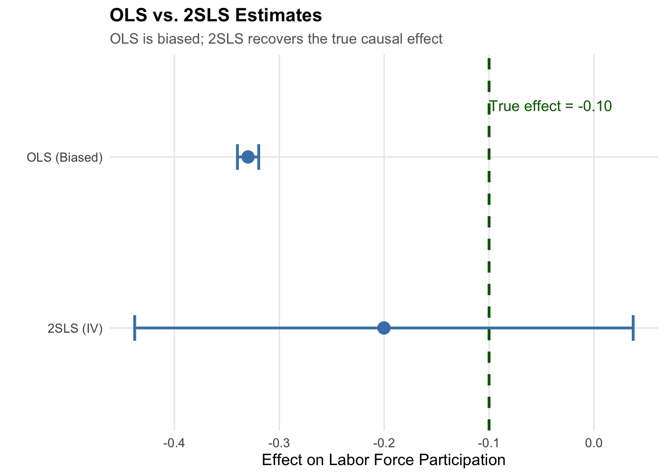

Figure 14.5: Comparing OLS (biased) and 2SLS (unbiased) estimates. OLS overstates the negative effect because career orientation confounds the relationship.

The OLS estimate is more negative than the true effect (-0.10) because it’s contaminated by selection: women with lower career orientation both have more children and are less likely to work, making the correlation more negative than the causal effect.

The 2SLS estimate is much closer to the true effect because it uses only the exogenous variation from the same-sex instrument.

14.5 Testing for Weak Instruments

14.5.1 The Weak Instrument Problem

If the instrument is only weakly correlated with \(X\), 2SLS performs poorly:

• Estimates become biased (toward OLS!)
• Standard errors become unreliable
• Inference is invalid

14.5.2 The First-Stage F-Test

The standard diagnostic for instrument strength is the first-stage F-statistic, which comes from the first-stage regression \[ X_i = \pi_0 + \pi_1 Z_i + \nu_i \] and tests the null \(H_0: \pi_1 = 0\) that the instruments have no predictive power for \(X\). With a single instrument, the first-stage F is just the square of the t-statistic on \(\pi_1\); with multiple instruments, it is the joint test that none of them predict \(X\). A large F means the instruments are collectively doing real work—they move \(X\) around a lot. feols() reports this statistic directly in its summary() output, or you can pull it out with fitstat(tsls, ~ ivf).

The traditional rule of thumb, following Stock and Yogo (2005), is that a first-stage F of at least 10 is enough to consider an instrument “strong.” That threshold has been the textbook standard for two decades. More recent work, however, suggests it is too lenient. Lee et al. (2022) show that the F-statistic needed to justify conventional t-test inference on the 2SLS coefficient is closer to 100 than to 10— so an instrument with, say, F = 20 may still produce fine point estimates, but its confidence intervals are likely too narrow. A safer modern default is to treat an F between 10 and roughly 100 with caution and to prefer much stronger first stages when they are available. In our running example the first-stage F is well into the hundreds, so the instrument clears both the classic and the modern bar comfortably.

14.5.3 What Happens with a Weak Instrument?

Let’s see what happens when we use a weak (essentially random) instrument:

# Create a weak instrument (random noise)
set.seed(123)
ae_sim <- ae_sim |>
    mutate(weak_instrument = rnorm(n()))

# Try 2SLS with weak instrument
weak_iv <- feols(mom_worked ~ 1 | 0 | morekids ~ weak_instrument,
                 data = ae_sim)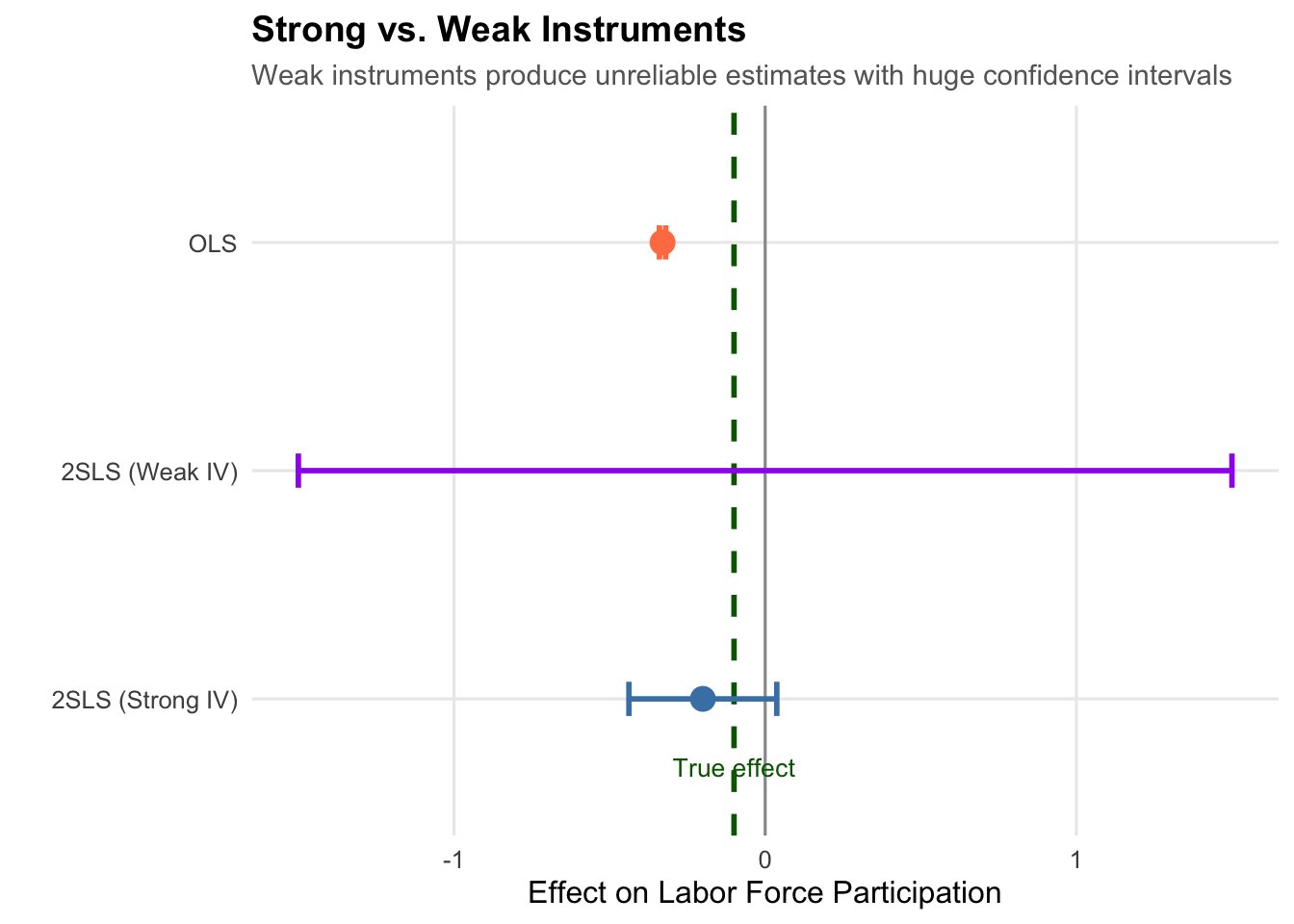

Figure 14.6: With a weak instrument (random noise), the 2SLS estimate becomes unreliable with huge standard errors.

With a weak instrument, the estimate is wildly off and the confidence interval is enormous. Always check your first-stage F-statistic!

14.6 What Does IV Estimate? The LATE

14.6.1 The Local Average Treatment Effect

An important subtlety: IV does not estimate the same quantity as OLS or DiD. It estimates the Local Average Treatment Effect (LATE)—the causal effect for a specific subpopulation called compliers.

14.6.2 Four Types of People

In the fertility example, we can categorize people by how their fertility responds to the instrument:

Type	Description
Always-takers	Would have 3+ kids regardless of sex composition
Never-takers	Would never have 3+ kids regardless of sex composition
Compliers	Have 3+ kids because first two were same-sex
Defiers	Have 3+ kids only if first two were different-sex

IV identifies the causal effect only for compliers—those whose treatment status was actually changed by the instrument.

14.6.3 Who Are the Compliers?

In the Angrist-Evans context, compliers are parents who:

• Wanted mixed-sex children strongly enough to try for a third
• Would have stopped at two kids if the first two were different sexes

This is not:

• All parents with 3+ children
• Parents who wanted large families regardless
• Parents who strongly preferred small families

14.6.4 Trade-offs of IV Estimation

Advantages	Disadvantages
Credible causal identification	Estimates LATE, not ATE
Handles endogeneity	Less generalizable
No need for RCT or natural experiment	Requires strong assumptions
Works with cross-sectional data	Often larger standard errors

14.7 Classic IV Applications

Instrumental variables have been used to study many important questions:

Study	Question	Instrument
Card (1995)	Returns to education	Distance to college
Acemoglu et al. (2001)	Do institutions cause growth?	Colonial settler mortality
Levitt (1997)	Effect of police on crime	Electoral timing
Angrist & Krueger (1991)	Returns to education	Quarter of birth

14.7.1 Example: Card (1995) - Returns to Education

Question: What is the causal effect of education on wages?

Problem: Ability is unobserved but affects both education and wages, biasing OLS upward.

Instrument: Distance to the nearest college. People who grew up closer to a college got more education.

Why relevant? Proximity reduces the cost of attending college.

Why excludable? Distance to a college shouldn’t directly affect wages decades later (only through education).

Finding: Returns to education are actually higher than OLS suggests—the ability bias works in the opposite direction from what many expected.

14.7.2 Example: Acemoglu, Johnson, & Robinson (2001) - Institutions and Growth

Question: Do institutions—property rights, rule of law, constraints on government—cause long-run economic growth?

Problem: Institutions and income are jointly determined. Rich countries can afford (and demand) better institutions in part because they are rich, so OLS confuses the effect of institutions on growth with the effect of growth on institutions. Unobserved factors like geography and culture correlate with both.

Instrument: Settler mortality rates faced by European colonizers in the 17th-19th centuries. Where Europeans faced high disease mortality (parts of sub-Saharan Africa, for instance), they set up “extractive” institutions designed to siphon resources rather than protect property. Where they could settle safely (North America, Australia, New Zealand), they transplanted European-style property-rights institutions. Those early institutional choices persisted for centuries.

Why relevant? Historical settler mortality strongly predicts modern institutional quality, because colonial institutional form carried forward through independence.

Why excludable? European mortality from disease hundreds of years ago should not directly affect a country’s GDP today except through the institutions it shaped. The relevant diseases (malaria, yellow fever) had much smaller effects on indigenous populations with partial immunity than on European newcomers.

Finding: Institutions have a large causal effect on GDP per capita; the IV estimate is larger than OLS. The paper sparked a broad “institutions vs. geography” debate in development economics.

14.7.3 Example: Levitt (1997) - Police and Crime

Question: Does hiring more police cause crime to fall?

Problem: Reverse causality. Cities with high crime hire more police in response, so OLS typically shows a positive correlation between police and crime— implying police increase crime, which is obviously backwards.

Instrument: The timing of mayoral and gubernatorial elections. Police hiring in U.S. cities spikes in the year before an election because incumbents want to campaign on being tough on crime.

Why relevant? Police staffing rises predictably in the run-up to elections, providing variation in police levels that is not driven by current crime trends.

Why excludable? The electoral calendar is set by state law, not by recent crime fluctuations. There is no obvious direct channel from “an election is approaching” to “less crime this year” except through its effect on police hiring.

Finding: Additional officers reduce crime substantially, and the IV estimate flips the sign of the naive OLS correlation. A coding error in the original paper was later flagged by McCrary (2002) and the estimates revised downward, but the qualitative conclusion—that more police reduce violent crime—survives.

14.7.4 Example: Angrist & Krueger (1991) - Quarter of Birth

Question: What is the causal return to education on earnings?

Problem: The same ability bias Card faces. Unobserved ability raises both schooling and wages, so OLS estimates of the return to education conflate education’s causal effect with the effect of being able.

Instrument: Quarter of birth. U.S. compulsory-schooling laws require children to start school the September of the year they turn 6, but allow them to drop out at 16. A child born in Q1 starts school older and hits the dropout age with less time in school; a child born in Q4 starts younger and is forced to stay in longer before becoming legally allowed to leave. People born late in the year therefore attain slightly more education, on average, than people born early in the year.

Why relevant? First-stage regressions show a detectable (though modest) relationship between quarter of birth and total years of schooling.

Why excludable? Quarter of birth should be essentially random with respect to ability, family background, and earnings potential. There is no obvious reason being born in January rather than October would directly affect adult wages other than through education.

Finding: Returns to education estimated by IV are close to OLS, suggesting ability bias may be smaller than many feared. Later work (Bound et al. 1995) cautioned that quarter of birth is actually a fairly weak instrument— in fact, Angrist-Krueger is often cited as a motivating example for the weak-instrument literature we discussed in the previous section.

14.8 Summary

Instrumental variables provide a powerful tool for causal inference when other methods fail. The key is finding a variable that affects treatment but has no direct effect on the outcome.

The two requirements:

1. Relevance: The instrument predicts the endogenous variable (testable via first-stage F-statistic > 10)
2. Exclusion: The instrument affects the outcome only through the treatment (requires economic reasoning—not directly testable)

Key insights:

• 2SLS uses only the exogenous variation in \(X\) induced by \(Z\)
• IV estimates the Local Average Treatment Effect (LATE) for compliers
• Weak instruments produce unreliable estimates—always check the first-stage F-statistic
• The exclusion restriction is crucial but untestable—think carefully about whether it holds

IV requires strong assumptions, but when those assumptions are credible, it provides a path to causal inference even in challenging observational settings.

14.9 Check Your Understanding

For each question below, select the best answer from the dropdown menu.

i. What does it mean for a variable to be "endogenous"? -- Select Answer -- The variable is measured with error The variable has a large variance The variable is correlated with the error term The variable is binary

ii. Which IV assumption can be directly tested? -- Select Answer -- Relevance (Z predicts X) Exclusion restriction (Z affects Y only through X) Both can be tested Neither can be tested

iii. In the Angrist-Evans study, why is same-sex a valid instrument for fertility? -- Select Answer -- Same-sex children are more expensive to raise Parents prefer mixed-sex children and try for another if they have same-sex Same-sex children make mothers more likely to work Same-sex is correlated with education

iv. What is the rule of thumb for detecting weak instruments? -- Select Answer -- R² > 0.5 in the first stage p-value < 0.05 on the instrument First-stage F-statistic > 100 First-stage F-statistic > 10

v. IV estimates the effect for which subpopulation? -- Select Answer -- Always-takers Compliers Never-takers The entire population

vi. (Challenge) If OLS shows a negative relationship between X and Y, but 2SLS shows no relationship, what might this suggest? -- Select Answer -- The instrument is weak The true effect is negative but larger than OLS suggests Selection bias was creating a spurious negative correlation; the true causal effect may be zero The exclusion restriction is violated

TipShow Explanation

1. Endogeneity means the explanatory variable is correlated with the error term: Cov(X, μ) ≠ 0. This violates the key OLS assumption and causes bias. Common sources include omitted variables, selection, and reverse causality.

2. Relevance (Cov(Z, X) ≠ 0) can be tested by regressing X on Z and checking the F-statistic. The exclusion restriction (Cov(Z, μ) = 0) cannot be directly tested because we don’t observe μ. It must be justified with economic reasoning.

3. Parents tend to prefer having children of both sexes. If their first two children are the same sex, they’re more likely to try for a third to “get” the other sex. Since biological sex is essentially random, this creates exogenous variation in fertility.

4. Stock and Yogo (2005) established that a first-stage F-statistic below 10 indicates a weak instrument. With weak instruments, 2SLS estimates are biased (toward OLS) and inference is unreliable.

5. IV estimates the Local Average Treatment Effect (LATE) for compliers—those whose treatment status was actually changed by the instrument. It doesn’t identify effects for always-takers or never-takers, whose treatment status is unaffected by the instrument.

6. This pattern suggests that the OLS relationship was driven by selection or omitted variable bias rather than a true causal effect. For example, if people who choose X also have characteristics that lead to lower Y, OLS would show a negative correlation even if X has no causal effect. 2SLS, by using only exogenous variation, reveals that the true causal effect is zero.

Angrist, Joshua D., and William N. Evans. 1998. “Children and Their Parents’ Labor Supply: Evidence from Exogenous Variation in Family Size.” American Economic Review 88 (3): 450–77. https://www.jstor.org/stable/116844.

Bound, John, David A. Jaeger, and Regina M. Baker. 1995. “Problems with Instrumental Variables Estimation When the Correlation Between the Instruments and the Endogenous Explanatory Variable Is Weak.” Journal of the American Statistical Association 90 (430): 443–50. https://doi.org/10.2307/2291055.

Lee, David S., Justin McCrary, Marcelo J. Moreira, and Jack Porter. 2022. “Valid t-Ratio Inference for IV.” American Economic Review 112 (10): 3260–90. https://doi.org/10.1257/aer.20211063.

McCrary, Justin. 2002. “Using Electoral Cycles in Police Hiring to Estimate the Effect of Police on Crime: Comment.” American Economic Review 92 (4): 1236–43. https://doi.org/10.1257/000282802762024610.

Stock, James H., and Motohiro Yogo. 2005. “Testing for Weak Instruments in Linear IV Regression.” In Identification and Inference for Econometric Models: Essays in Honor of Thomas Rothenberg, edited by Donald W. K. Andrews and James H. Stock. Cambridge University Press.